Architecting for Stability- Pre-Normalization, RMSNorm, and Mixed-Precision Training
Architecting for Stability: Pre-Normalization, RMSNorm, and Mixed-Precision Training
The Transformer architecture has been the catalyst for the most significant breakthroughs in artificial intelligence, but its original design presented notable training instabilities. Over time, the community has iterated on the architecture, leading to a de facto standard that is more robust and efficient.
This article explores the critical components of the modern Transformer block, focusing on the techniques that enable stable and high-performance training. We cover the shift to Pre-Normalization, the role of Root Mean Square Layer Normalization (RMSNorm), and how these concepts elegantly map to the specialized hardware of modern GPUs for low-precision training.
1. The Pre-Normalization Paradigm
A key evolution from the original Transformer was the repositioning of the layer normalization. This seemingly small change has a profound impact on gradient flow and overall training stability.
- Post-Normalization (Original Design): In the initial architecture, layer normalization was applied after the residual connection. This meant that the main branch of the network accumulated outputs from successive layers, potentially leading to a large variance that could cause exploding or vanishing gradients, especially in deep models.
# Post-Norm Block Flow
sublayer_output = Sublayer(input)
added_output = input + sublayer_output
output = LayerNorm(added_output)
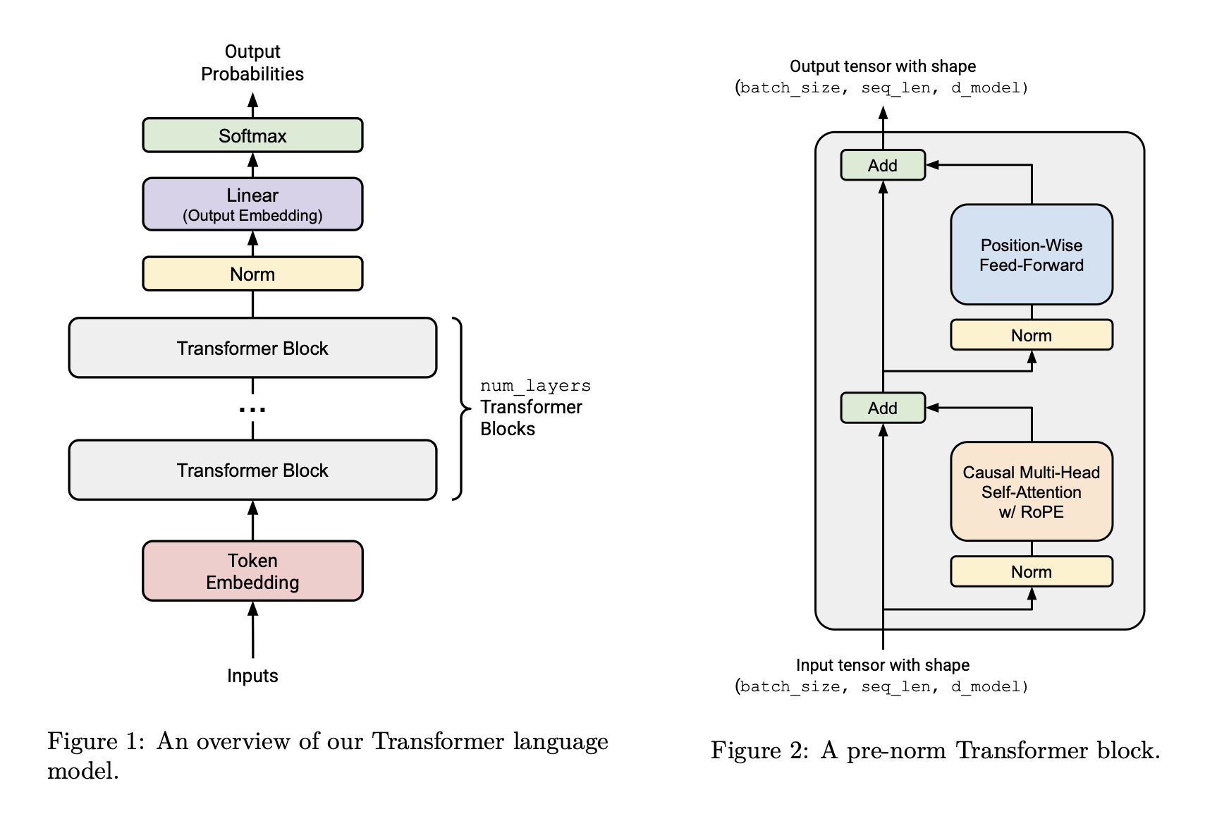
- Pre-Normalization (Modern Design): In this paradigm, layer normalization is applied to the input before it enters a sub-layer. The residual connection then bypasses the normalization layer. This ensures that the signal passed into each sub-layer (Self-Attention or the Feed-Forward Network) is consistently scaled, leading to a more stable optimization landscape.
# Pre-Norm Block Flow
normalized_input = LayerNorm(input)
sublayer_output = Sublayer(normalized_input)
output = input + sublayer_output
The Pre-Norm structure has become standard practice as it significantly improves training reliability and often reduces the need for extensive learning rate warm-up schedules.
2. RMSNorm: Efficient and Simplified Normalization
While standard Layer Normalization is effective, it can be simplified. Root Mean Square Layer Normalization (RMSNorm) does this by removing the mean-centering step (re-centering), focusing solely on re-scaling the norm of the activations. For a given input vector (x) of dimension (d), the RMSNorm is defined as:
[\text{RMS}(x) = \sqrt{\frac{1}{d}\sum_{i=1}^{d} x_i^2}]
[y = \frac{x}{\text{RMS}(x) + \epsilon} \cdot \gamma]
Where:
- x: The input vector, typically the features for a single token. Normalization is applied independently to each vector across this feature dimension.
- d: The dimensionality of the feature vector (
d_model). - γ (gamma): A learnable gain parameter vector that allows the network to adaptively scale the normalized output. It is typically initialized to ones.
- ε (epsilon): A small constant added to the denominator for numerical stability, preventing division by zero.
By omitting the mean calculation, RMSNorm reduces computation while performing comparably to, and in some cases better than, standard Layer Normalization.
3. The Challenge of Low-Precision Computation
To achieve maximum performance, modern deep learning relies on mixed-precision training, using low-precision formats like float16 or FP8 for the bulk of the computation. These formats drastically reduce memory footprint and leverage specialized hardware accelerators. However, their primary drawback is a significantly limited numerical range.
| Data Type | Maximum Value |
|---|---|
float16 |
65,504 |
float32 |
~3.4 x 10^38 |
This limitation poses a direct threat to the RMSNorm calculation. The first step involves squaring the input elements ((x_i^2)). Even a moderate input value can easily exceed the maximum range of a low-precision format when squared.
For example, if an input vector in float16 contains the value 300.0, the squaring operation yields 90,000.0, which is beyond the float16 limit. This results in numerical overflow, where the value is replaced by infinity. Any subsequent operation involving infinity will corrupt the entire calculation, leading to a meaningless output (often a vector of zeros or NaNs) and destabilizing training.
4. Hardware-Aware Implementation: Strategic Upcasting
The solution to this numerical challenge is not to abandon low-precision training, but to apply high precision strategically where it matters most. For sensitive element-wise operations like those in RMSNorm, the input is temporarily promoted to a more stable format.
This is achieved by upcasting the input tensor from its low-precision format (e.g., FP8 or float16) to float32 just for the duration of the normalization calculation.
# Conceptual implementation of RMSNorm with strategic upcasting
def stable_rms_norm(input: Tensor, weight: Tensor, eps: float) -> Tensor:

    # Preserve the original, low-precision dtype
    input_dtype = input.dtype

    # 1. Upcast to float32 for stable computation
    x = input.to(torch.float32)

    # 2. Perform squaring and other sensitive math in float32
    variance = x.pow(2).mean(dim=-1, keepdim=True)
    rsqrt = torch.rsqrt(variance + eps)
    normalized_x = x * rsqrt

    # 3. Apply gain and downcast back to the original dtype
    output = weight * normalized_x
    return output.to(input_dtype)
This software technique aligns with the architecture of modern GPUs like NVIDIA’s Hopper series:
- Massive Matrix Multiplications: The vast majority of a Transformer’s workload (e.g., in
Linearlayers and attention) are matrix multiplications. These are routed to highly specialized Tensor Cores, which execute these operations at immense speed using low-precision formats likeFP8. - Sensitive Element-Wise Operations: The calculations inside RMSNorm are not matrix multiplications. These are handled by the GPU’s general-purpose cores. The brief upcast to
float32ensures numerical stability for these operations before the result is downcast back toFP8and passed to the next layer for processing on the Tensor Cores.
This compute split—routing operations to the appropriate specialized hardware with the appropriate numerical precision—is fundamental to achieving both state-of-the-art performance and the stability required to train massive models.